ON THIS PAGE:
The Drift Detection Process monitors the deviation between process variable data (inputs) and a reference input. The reference input can either be a fixed value, or it can be a dynamic value such as an entity.
A primary deviation limit is applied to the reference input, as either a percentage value or an absolute value. This limit can be an upper limit, a lower limit, or both, forming a deviation band. In the same way, secondary and tertiary limits may be applied to the reference input, to raise secondary or tertiary states, respectively.
Upper and lower primary deviation limits are created:
 |
 |
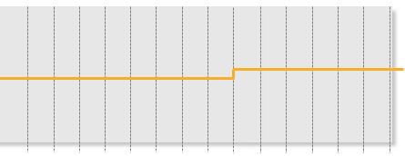
| The reference input data shown over several sample intervals |
Using an Absolute Value deviation mode, a primary deviation “band” is created. Upper and Lower deviations are used in this example. |
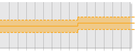
Input Data is evaluated against upper and lower primary deviation limits:
 |
|
| Input data is evaluated against the primary deviation limits at every sample interval. |
As well as detecting data that breaches the primary, secondary and tertiary deviation limits (raising a primary, secondary or tertiary state, respectively), the drift detection process has a variety of option methods for raising a secondary or tertiary event.
The Drift Detection process can measure duration above the primary limit, and also the number of data points above the primary limit. These measurements can be taken consecutively, or they can be summed in total over the preceding rolling sum period.
The Drift Detection process is used for monitoring the deviation between a reference input and the test input. Unacceptable deviations may signify equipment failure or calibration errors.
Drift Detection is a complex process capable of concurrently monitoring multiple conditions such as transgression of limits, state duration, and movement between states.
State Transition Rules
The Drift Detection process has clearly defined state transition logic paths. Transition from one state to another is equally dependant on the current evaluation of data, and on the current state.
State transitions cause events to be raised, allowing for the escalation of actions via the Sentinel framework. Different actions can be assigned to different state outcomes.
The following table outlines the allowable state transitions of the Drift Detection process.
| This state can transition | To this state | Under these conditions |
| Default | Primary | Data has transgressed the primary state upper or lower deviation limits. |
| Primary | Secondary | Any one of the secondary state conditions have been met. |
| Tertiary | Only if the tertiary deviation limit is breached. | |
| Default | Data is not erroneous, and is within the deviation limits of the curve. | |
| Secondary | Tertiary | Any one of the tertiary state conditions has been met. |
| Default | Data is not erroneous, and is within the deviation limits of the curve. | |
| Tertiary | Default | Data is not erroneous, and is within the deviation limits of the curve. |
The following diagram outlines the state transition logic of the Drift Detection process.
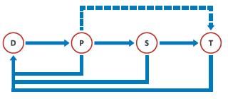 |
D Default P Primary S Secondary T Tertiary |
Test Outcomes
A number of outcomes are possible when the Drift Detection process is executed:
| Default State | Data is not in an erroneous state and is within the primary deviation limits. |
| Primary State | Data is measured against the defined fixed or variable primary deviation limit (upper and/or lower). If it breaches a primary deviation limit, a primary state is reached, and a primary event is raised. |
| Secondary State | A number of possible conditions can cause a secondary event, leading to a secondary state. These are explained in more detail in the Secondary State section. |
| Tertiary State | As with the secondary state, a number of conditions can cause a tertiary event. These are explained in more detail in the Tertiary State section. |
| Suppressed State | The monitor has been suppressed. For example, if the precondition has not been met. |
Conditional Logic
The Drift Detection process provides the following conditional logic.
Note: All of the example graphs in the following sections show tests that have used the Last Known Value sample method.
Input Settings
The input and the reference input are defined in this section.
- Input: The input is the data that is monitored. Input data is defined as an attribute of the source entity, either as it is, or as part of a calculation.
- Reference Input: The fixed or variable reference input is used to create deviation limits for the input data. The process will calculate limits around the reference input based on the deviation mode and the deviation limit settings, and then compare the input data stream to this model in order to determine drift.
Mode Settings
Define whether the deviation mode is a percentage or an absolute value, to establish how primary, secondary and tertiary deviation limits are calculated. Also select whether to set upper or lower deviation limits, or both.
Deviation Limit Settings
The primary state deviation limit must be set for the process to work. If the calculated primary state deviation limit is breached, a primary event occurs, and a primary state is reached. Optionally, a secondary state deviation limit and a tertiary state deviation limit may be set for the process.
Rolling Sum Period
A secondary state rolling sum period can be defined for evaluating some of the secondary state conditions; likewise, a tertiary state rolling sum period can be defined for evaluating some of the tertiary state conditions.
The rolling sum period is a defined period (specified in days and hours). At every sample interval, the rolling sum period is that period preceding the sample interval. So, for example, if the secondary state rolling sum period is set at 1 day 2 hours then at 3pm on Tuesday 15 January 2013, the secondary state rolling sum period is from 1pm on Monday 14 January (covering the last 1 day and 2 hours). Any evaluations relating to that sample interval's secondary state rolling sum period conditions must fall within that time.
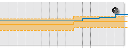
Primary State Deviation Limit
The primary state deviation limit must be set for the process to work.
If the configured primary state deviation limit is breached, a primary event occurs, and a primary state is reached.
Example:
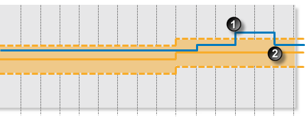
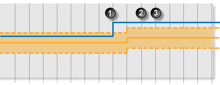
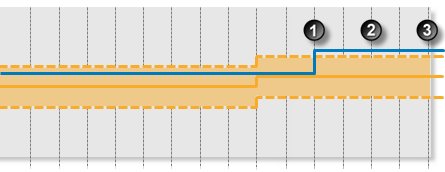
In this example, a primary event is raised when the input data breaches the upper primary deviation limit. The sample interval is one hour.
 |
|
|
Secondary State
There are several possible ways to reach the secondary state outcome in the Drift Detection process:
- Secondary State Deviation Limit
- Secondary State Duration Limit
- Secondary State Sustained Value Limit
- Secondary State Rolling Sum Total Duration Limit
- Secondary State Rolling Sum Breach Occurrences Limit
You can choose to set one or more conditions to trigger the secondary state. For example, a test may have a secondary deviation limit defined, as well as configured variables for determining secondary state rolling sum breach occurrences.
Deviation Limit
If the configured secondary deviation limit is breached, a secondary event occurs, and a secondary state is reached.
Example:
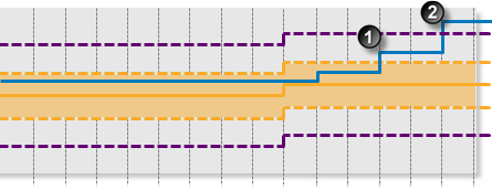
In this example, a secondary event is raised when the input data breaches the upper secondary deviation limit. The sample interval is one hour.
 |
|
|
Duration Limit
Monitor for data that continuously exceeds the primary deviation limit, for longer than the secondary state duration limit.
If data that continuously exceeds the primary deviation limit for longer than specified in the secondary state duration limit, a secondary event occurs, and a secondary state is reached.
Example:
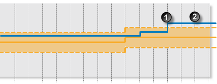
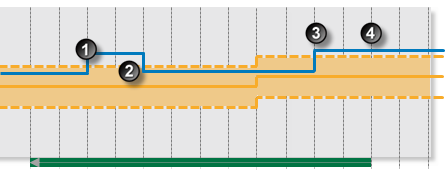
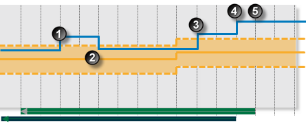
In this example, a secondary event is raised when the input data has exceeded the upper primary deviation limit for a period of 2 hours, exceeding the primary state duration limit of 1.5 hours. The sample interval is one hour.
 |
|
|
Sustained Value Limit
Monitor for when data exceeds the primary deviation limit for more than a specified number of times (secondary state, sustained value limit), consecutively. When this happens, a secondary event occurs, and a secondary state is reached.
Example:
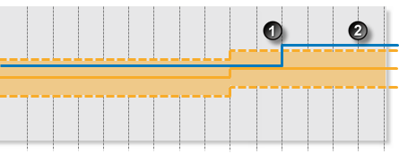
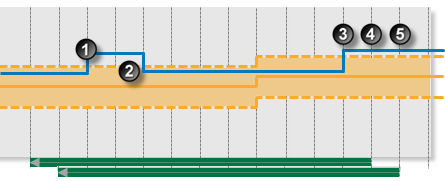
In this example, a secondary event is raised when the input data has exceeded the upper deviation limit, consecutively, for four sample intervals, exceeding the secondary state sustained value limit of 3. The sample interval is one hour.
|
|
|
|
|
Rolling Sum Total Duration Limit
Monitor for a specified accumulated duration of all periods where data is in breach of the primary deviation limit, within the preceding specified secondary state rolling sum period.
If the total combined primary state duration is longer than the specified secondary state rolling sum duration limit, a secondary event occurs, and a secondary state is reached.
Example:
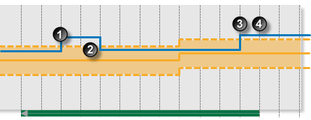
In this example, a secondary event is raised when the input data is above the primary deviation limit for a total of four hours during the current secondary state rolling sum period, exceeding the secondary state rolling sum duration limit of 3.5 hours. The sample interval is one hour. Secondary state rolling sum period is 12 hours.
 |
|
|
Rolling Sum Breach Occurrences Limit
Monitor for when a set number of values (secondary state breach occurrences limit) has breached the primary deviation limit, during the preceding specified secondary rolling sum period.
Example:
In this example, a secondary event is raised when the input data has breached the primary deviation limit three times in the current secondary state rolling sum period, reaching the secondary state rolling sum breach occurrences limit of 3. The sample interval is one hour. Secondary state rolling sum period is 12 hours.
 |
|
|
Tertiary State
There are several ways to reach the tertiary state outcome in the Drift Detection process:
- Tertiary State Deviation Limit
- Tertiary State Duration Limit
- Tertiary State Sustained Value Limit
- Tertiary State Rolling Sum Total Duration Limit
- Tertiary State Rolling Sum Breach Occurrences Limit
You can choose to set one or more conditions to trigger the tertiary state. For example, a test may have a tertiary deviation limit defined, as well as configured variables for determining tertiary state rolling sum breach occurrences.
Deviation Limit
If the configured tertiary deviation limit is breached, a tertiary event occurs, and a tertiary state is reached.
The graph demonstrates a breach of the tertiary deviation limit, causing a tertiary event to occur.
Example:
In this example, a tertiary event is raised when the input data breaches the upper tertiary deviation limit. The sample interval is one hour.
 |
|
|
Duration Limit
Monitor for data that continuously exceeds the primary deviation limit, for longer than the tertiary state duration limit.
If data that continuously exceeds the primary deviation limit for longer than specified in the tertiary state duration limit, a tertiary event occurs, and a tertiary state is reached.
Example:
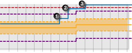
In this example, a tertiary event is raised when the input data has exceeded the upper primary deviation limit consecutively for a period of 3 hours, exceeding the tertiary state duration limit of 2.5 hours. Secondary state duration limit is 1.5 hours. The sample interval is one hour.
 |
|
|
Sustained Value Limit
Monitor for when data exceeds the primary deviation limit for more than a specified number of times (tertiary state sustained value limit), consecutively. If this is the case, a tertiary event occurs, and a tertiary state is reached.
Example:
In this example, a tertiary event is raised when the input data has exceeded the upper deviation limit for five sample intervals, consecutively, exceeding the tertiary state sustained value limit of 4. Secondary state sustained value limit is 2. The sample interval is one hour.
 |
|
|
Rolling Sum Total Duration Limit
Monitor for a specified accumulated duration of all periods where data is in breach of the primary deviation limit, within the preceding specified tertiary state rolling sum period.
If the total combined primary state duration is longer than the specified tertiary state rolling sum duration limit, a tertiary event occurs, and a tertiary state is reached.
Example:
In this example, the tertiary state rolling sum duration limit is exceeded, causing a tertiary event. Tertiary state rolling sum total duration is 3.5 hours. Tertiary rolling sum period is 12. The sample interval is one hour.
 |
|
|
Rolling Sum Breach Occurrences Limit
Monitor whether a set number of values (tertiary state breach occurrences limit) has breached the primary deviation limit, during the preceding specified tertiary rolling sum period.
Example:
In the following example, the tertiary state rolling sum breach occurrences limit is exceeded, causing a tertiary event. Note that a secondary state must be reached first. Tertiary state breach occurrences limit is 3. Tertiary rolling sum period is 12 hours. The sample interval is 1 hour.
 |
|
|
Adding a Drift Detection Process
The Drift Detection Process monitors the deviation between process variable data (inputs) and a reference input. If a limit or condition is breached when the process is executed, a new state is reached and an event is raised.
Setting Process Values and Limits
Part of setting up the Drift Detection process involves selecting limits, such as the primary state deviation limit, secondary state deviation limit, tertiary state deviation limit, breach occurrences limits and so on. Limits can either be fixed values, or they can be variable data taken from entities.
The following limits are available. Select a limit type from the drop-down list, then type in or select a limit.
- Fixed Value: Type in a numerical value.
- Attribute: This option is only available if the test’s Source Type is Entity or Hierarchy.
Click the ellipsis button to select an attribute of the source entities.
 - Source Tag: This option is only available if the Source Type is Tag.
- Calculation: Click the ellipsis
 button to open the Edit Calculation window.
- If the Source Type is Entity or Hierarchy: Type a calculation, prefixed by ‘this’ as the Source Entity token, for example: {this:THP} + 34.
- If the Source Type is Tag: Type a calculation, prefixed by ‘this’ as the Source Tag token, for example: {this} * 2.
- Tag: Click the ellipsis
 button to select a tag.
 - Entity Attribute: Click the ellipsis
 button to select an entity. From here, select an attribute, or attribute value, for the selected entity.
Adding the Process
As with all Sentinel processes, the Drift Detection Process is defined within a Sentinel Test page.
In the Sentinel Test page:
1. Expand the Process ![]() panel.
panel.
2. Select Drift Detection from the drop-down list.
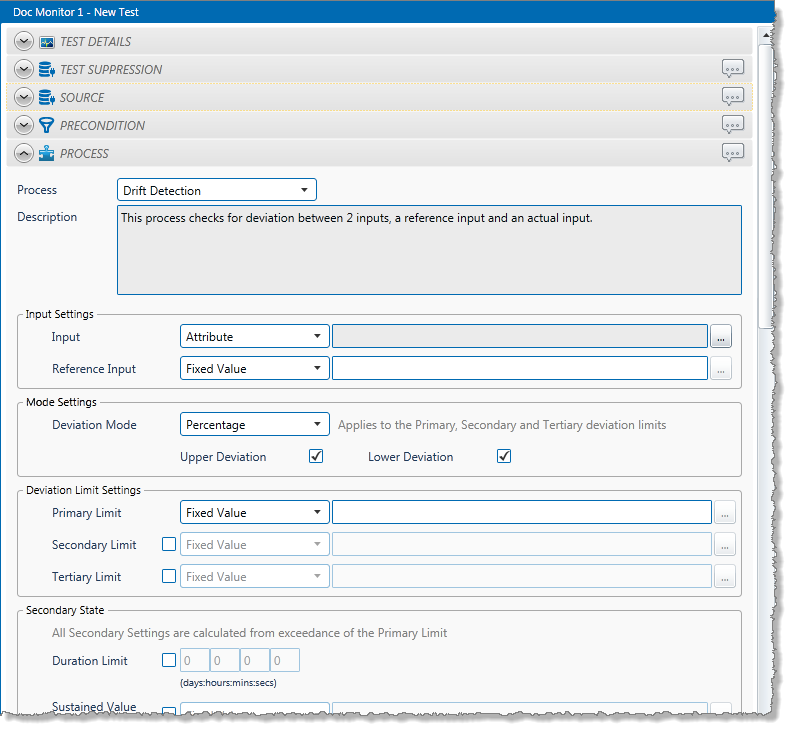
Input Settings
3. From the Input drop-down list, select an input from the following:
- Attribute: This option is only available if the Source Type is Entity or Hierarchy.
Click the ellipsis button to select an attribute. You are limited to selecting an attribute of the test source monitor items. This attribute of each of the monitor items is a separate process input.
 - Source Tag: This option is only available if the Source Type is Tag.
- Calculation: Click the ellipsis
 button to open the Edit Calculation window.
- If the Source Type is Entity or Hierarchy: Type a calculation, prefixed by ‘this’ as the Source Entity token, for example: {this:THP} + 34.
- If the Source Type is Tag: Type a calculation, prefixed by ‘this’ as the Source Tag token, for example: {this} * 2.
- Entity Attribute: Click the ellipsis
 button to select an entity. From here, select an attribute, or attribute value, for the selected entity.
4. From the Reference Input drop-down list, select one of the following; then type in or select a corresponding value:
- Fixed Value
- Attribute (only available of the Source type is Entity or Hierarchy)
- Source Tag (only available of the Source type is Tag)
- Calculation
- Tag
- Entity Attribute
Mode Settings
5. Define whether the deviation mode is a percentage or an absolute value, to establish how primary, secondary and tertiary deviation limits are calculated. Also select whether to set upper or lower deviation limits, or both.
Note: The mode settings apply to primary, secondary and tertiary deviation limits.
- From the Deviation Mode drop-down list, select Percentage or Absolute Value. The deviation mode determines how the deviation limits will be calculated.
- Select the Upper Deviation check box to set an upper deviation limit.
- Select the Lower Deviation check box to set a lower deviation limit.
Deviation Limit Settings
Note: The Primary Deviation Limit is mandatory for the Drift Detection Process.
6. From the Primary Limit drop-down list, select one of the following and then type in or select a corresponding value:
- Fixed Value
- Attribute (only available of the Source type is Entity or Hierarchy)
- Source Tag (only available of the Source type is Tag)
- Calculation
- Tag
- Entity Attribute
7. Optionally define secondary limits in the same way (first select the Secondary Limit check box).
8. Optionally define tertiary limits in the same way (first select the Tertiary Limit check box).
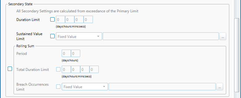
Secondary State
Note: All Secondary State settings are calculated from the primary deviation limit.
All secondary state settings are captured or selected in the Secondary State section of the process, with the exception of the Secondary Deviation Limit, which is set in the Deviation Limit Settings section of the process.
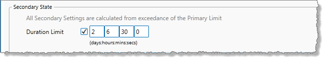
Duration Limit
The Secondary State Duration Limit is used for monitoring where data is continuously beyond the primary deviation limit, for longer than the specified secondary duration limit.
9. In the Secondary State section:
- Select the Duration Limit check box.
- Type integer values in the days, hours, mins (minutes), and secs (seconds) Duration Limit boxes to define a duration period. The default value is zero.
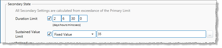
Sustained Value Limit
The Secondary State Sustained Value Limit is used for monitoring where data is beyond the primary deviation limit for more than a specified number of times (secondary state sustained value limit), consecutively.
10. In the Secondary State section:
- Select the Sustained Value Limit check box.
- From the Sustained Value Limit drop-down list, select one of the following and then type in or select a corresponding value:
-
- Fixed Value
- Attribute (only available of the Source type is Entity or Hierarchy)
- Source Tag (only available of the Source type is Tag)
- Calculation
- Tag
- Entity Attribute
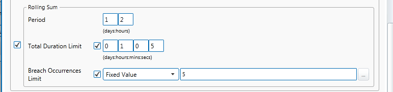
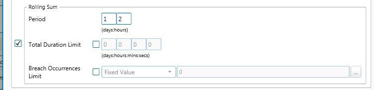
Rolling Sum Period
The rolling sum period is a defined period (specified in days and hours). At every sample interval, the rolling sum period applies to that period preceding the sample interval.
Set a secondary state rolling sum period if you are going to define a Secondary State Total Duration Limit or a Secondary State Breach Occurrences Limit.
11. In the Secondary State section:
- Select the check box to the left of the Rolling Sum section.
- Type integer values in the days and hours Period boxes to define the rolling sum period.

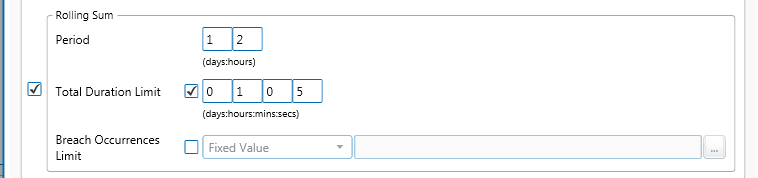
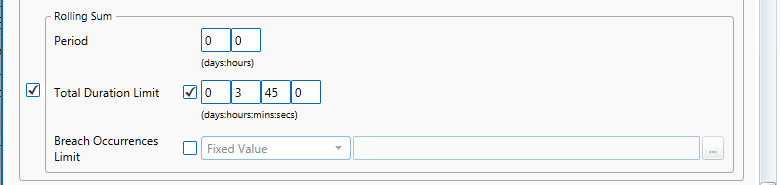
Rolling Sum Total Duration Limit
The Secondary State Rolling Sum Total Duration Limit is used to monitor for a specified accumulated duration of all periods where data is in breach of the primary deviation limit, within the preceding specified secondary state rolling sum period.
12. In the Rolling Sum section, within the Secondary State section:
- Select the Total Duration Limit check box.
- Type integer values in the days, hours, mins (minutes), and secs (seconds) Total Duration Limit boxes to define a total duration limit period. The default value is zero.
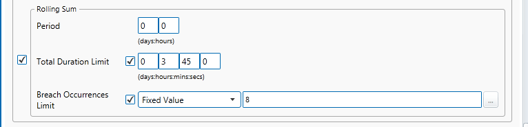
Rolling Sum Breach Occurrences Limit
The Secondary State Rolling Sum Breach Occurrences Limit is used to monitor for when a set number of values (secondary state breach occurrences limit) has breached the primary deviation limit, during the preceding specified secondary state rolling sum period.
13. In the Rolling Sum section, within the Secondary State section:
- Select the Breach Occurrences Limit check box.
- From the Breach Occurrences Limit drop-down list, select one of the following and then type in or select a corresponding value:
-
- Fixed Value
- Attribute (only available of the Source type is Entity or Hierarchy)
- Source Tag (only available of the Source type is Tag)
- Calculation
- Tag
- Entity Attribute
Tertiary State
Note: All Tertiary State settings are calculated from the primary deviation limit.
All tertiary state settings are captured or selected in the Tertiary State section of the process, with the exception of the Tertiary Deviation Limit which is set in the Deviation Limit Settings section of the process.
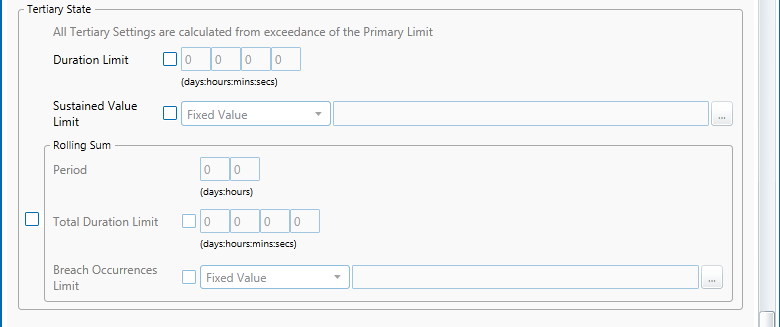
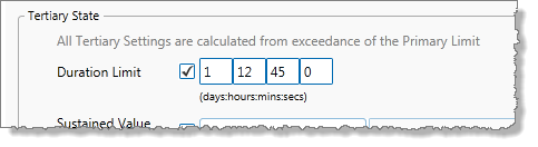
Duration Limit
The tertiary state duration limit is used for monitoring where data is continuously beyond the primary deviation limit, for longer than the specified tertiary duration limit.
14. In the Tertiary State section:
- Select the Duration Limit check box.
- Type integer values in the days, hours, mins (minutes), and secs (seconds) Duration Limit boxes to define a duration period. The default value is zero.
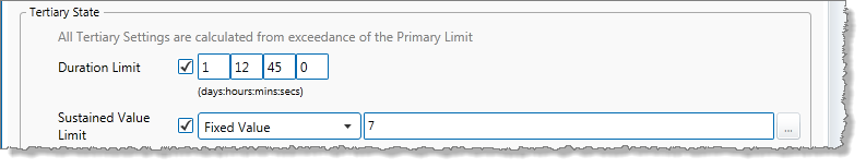
Sustained Value Limit
The Tertiary Sustained Value Limit is used for monitoring where data is beyond the primary deviation limit for more than a specified number of times (tertiary state sustained value limit), consecutively.
15. In the Tertiary State section:
- Select the Sustained Value Limit check box.
- From the Sustained Value Limit drop-down list, select one of the following and then type in or select a corresponding value:
-
- Fixed Value
- Attribute (only available of the Source type is Entity or Hierarchy)
- Source Tag (only available of the Source type is Tag)
- Calculation
- Tag
- Entity Attribute
Rolling Sum Period
The rolling sum period is a defined period (specified in days and hours). At every sample interval, the rolling sum period applies to that period preceding the sample interval.
Set a tertiary state rolling sum period if you are going to define a Tertiary State Total Duration Limit or a Tertiary State Breach Occurrences Limit.
16. In the Tertiary State section:
- Select the check box to the left of the Rolling Sum section.
- Type integer values in the days and hours Period boxes to define the rolling sum period. The default value is zero.
Rolling Sum Total Duration Limit
The Tertiary State Rolling Sum Total Duration Limit is used to monitor for a specified accumulated duration of all periods where data is in breach of the primary deviation limit, within the preceding specified tertiary state rolling sum period.
17. In the Rolling Sum section, within the Tertiary State section:
- Select the Total Duration Limit check box.
- Type integer values in the days, hours, mins (minutes), and secs (seconds) Total Duration Limit boxes to define a total duration limit period. The default value is zero.
Rolling Sum Breach Occurrences Limit
The Tertiary State Rolling Sum Breach Occurrences Limit is used to monitor for when a set number of values (tertiary state breach occurrences limit) has breached the primary deviation limit, during the preceding specified tertiary rolling sum period.
18. In the Rolling Sum section, within the Tertiary State section:
- Select the Breach Occurrences Limit check box.
- From the Breach Occurrences Limit drop-down list, select one of the following and then type in or select a corresponding value:
- Fixed Value
- Attribute (only available of the Source type is Entity or Hierarchy)
- Source Tag (only available of the Source type is Tag)
- Calculation
- Tag
- Entity Attribute
Adding Comments
19. To add comments to the process panel click the comment ![]() button, at the top right of the panel.
button, at the top right of the panel.
Configuring States
For the Drift Detection process, you can configure the following states, each with an optional state override and comments:
- Primary
- Secondary
- Tertiary
- Suppressed
You cannot change the severity of the Default state; however, you can add a state override and comments.
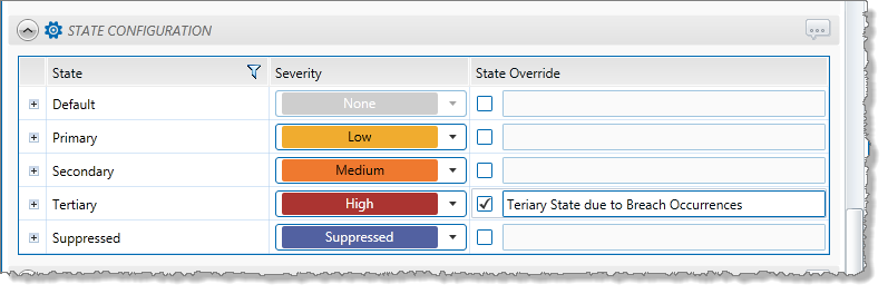
Note: Only configure states where you have set a limit.