ON THIS PAGE:
The Performance Curve process compares process variable data against limits and conditions that are defined by a performance curve. The performance curve uses a polynomial equation with coefficient and constant values from either fixed values or entities, or a combination of both.
Performance Curve is a complex process capable of concurrently monitoring multiple conditions such as transgression of limits, state duration, and movement between states.
State Transition Rules
The Performance Curve process has clearly defined state transition logic paths. Transition from one state to another is equally dependent on the current evaluation of data, and on the current state.
State transitions cause events to be raised, allowing for the escalation of actions via the Sentinel framework. Different actions can be assigned to different state outcomes.
The following table outlines the allowable state transitions of the Performance Curve process.
| This state can transition | To this state | Under these conditions |
| Default | Primary | Data has transgressed the primary state upper or lower deviation limits. |
| Out of Range | The x value of the data is not within the range defined by Min X and Max X. | |
| Primary | Secondary | Any of the secondary state conditions have been met. |
| Tertiary | Only if the tertiary deviation limit is breached. | |
| Default | Data is not erroneous, and is within the deviation limits of the curve. | |
| Secondary | Tertiary | Any of the tertiary state conditions has been met. |
| Default | Data is not erroneous, and is within the deviation limits of the curve. | |
| Out of Range | The x value of the data is not within the range defined by Min X and Max X. | |
| Tertiary | Default | Data is not erroneous, and is within the deviation limits of the curve. |
| Out of Range | The x value of the data is not within the range defined by Min X and Max X. | |
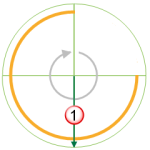
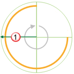
| Out of Range | Default | When data comes out of an Out of Range state, the state transition logic is applied to whatever the previous state was. So if, for example, the previous state was the primary state, a secondary state can be reached if any of the secondary state conditions have been met. |
| Primary | ||
| Secondary | ||
| Tertiary |
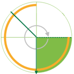
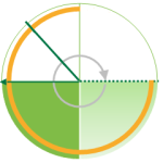
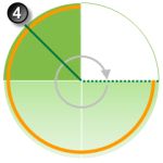
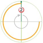
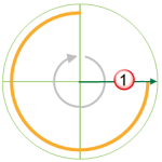
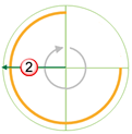
The following diagram outlines the state transition logic of the Performance Curve process.
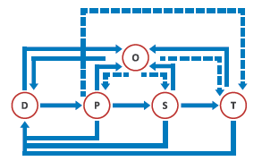 |
D Default P Primary S Secondary T Tertiary O Out of Range |
Test Outcomes
A number of outcomes are possible when the Performance Curve process is executed:
| Default State | Data is not in an erroneous state and is within the operating envelope. |
| Primary State | Data is measured against the defined fixed or variable primary deviation limit (upper and/or lower). If it breaches a primary deviation limit, a primary state is reached, and a primary event is raised. |
| Secondary State | A number of possible conditions can cause a secondary state. These are explained in more detail in the Secondary State section. |
| Tertiary State | As with the secondary state, a number of conditions can cause a tertiary state. These are explained in more detail in the Tertiary State section. |
| Out of Range State | When the X coordinate of the data falls outside the range defined by Min X and Max X, and Out of Range State is reached. This is explained in more detail in the Out of Range State section. |
| Suppressed State | The monitor has been suppressed. For example, if the precondition has not been met. |
Conditional Logic
The Performance Curve process provides the following conditional logic.
Note: All of the example graphs in the following sections show tests that have used the Last Known Value sample method.
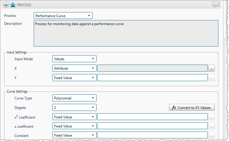
Input Settings
Depending on which Input Mode is selected, you will need to define various other input settings.
Choose between the Values input mode (where both the x and the y parameters can be fixed values or variable entities), and the Liquid Control Valve input mode.
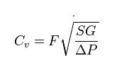
- Liquid Control Valve: The specialised Liquid Control Valve input mode uses the Flow Coefficient Equation (see diagram below) to calculate the Y value, based on specified (fixed or variable) values for: Flow Rate (F), Specific Gravity (SG) and Pressure Drop (P).
- Values: The Values input mode is used when you are not specifically measuring a Liquid Control Valve.
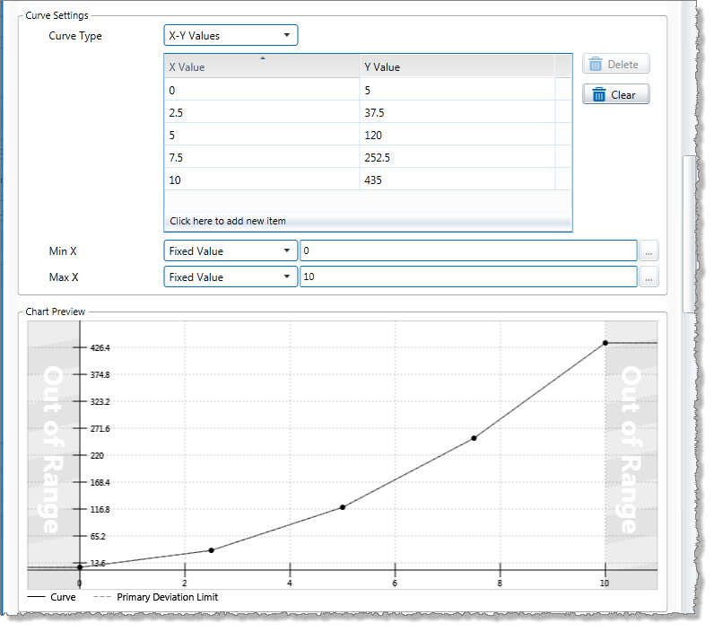
Curve Settings
Choose between the X-Y Values curve type, where a fixed, limited list of x and y values are manually captured, and the Polynomial curve type.
The Polynomial curve uses coordinates that are calculated at every sample interval, based on the x and y (fixed or variable) input values, creating a potentially varying range of deviation limits, whereas the X-Y Values creates a static set of limits that is the same at every sample interval. Polynomials can be set from zero (straight line), to nine degrees (more complex curve). Coordinates to the polynomial equation can also be fixed or variable.
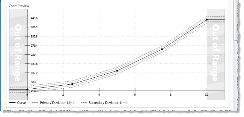
- Min X and Max X: Define out of range limits for the x value of the data.
- Chart Preview: The Performance Curve uses a graph to map out values based on the selected formula with the specified deviations.
Use the Convert to XY Values functionality to help with adjusting the polynomial curves.
For a polynomial curve type, if the process uses a hierarchy as the process source and an entity in the curve settings, you can select which entity to preview in the chart.
Mode Settings
Define whether the deviation mode is a percentage or an absolute value, to establish how primary, secondary and tertiary deviation limits are calculated. Also select whether to set upper or lower deviation limits, or both.
Rolling Sum Period
A secondary state rolling sum period can be defined for evaluating some of the secondary state conditions; likewise, a tertiary state rolling sum period can be defined for evaluating some of the tertiary state conditions.
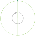
The rolling sum period is a defined period (specified in days and hours). At every sample interval, the rolling sum period is that period preceding the sample interval. So, for example, if the secondary state rolling sum period is set at 1 day 2 hours then at 3pm on Tuesday 15 January 2013, the secondary state rolling sum period is from 1pm on Monday 14 January (covering the last 1 day and 2 hours). Any evaluations relating to that sample interval's secondary state rolling sum period conditions must fall within that time.
Primary State Deviation Limit
The primary state deviation limit must be set for the process to work.
If the configured primary state deviation limit is breached, a primary event occurs, and a primary state is reached.
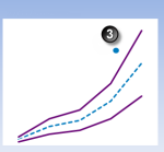
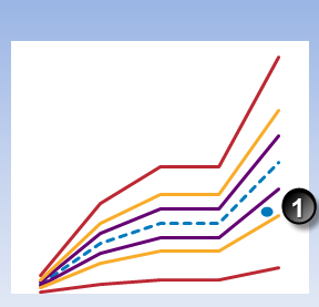
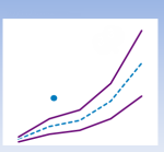
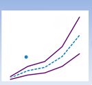
Example
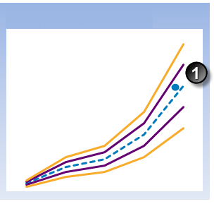
The following chart demonstrates a breach of the primary deviation limit, causing a primary event to occur.
- Input mode is values.
- Deviation mode is percentage.
- Limits are set for upper deviation and lower deviation.
- Curve settings are X-Y values; that is, they are static.
- The sample interval is every two hours.
 |
 |
 |
A default state is reached, and a default event is raised. |
Secondary State
There are several possible ways to reach the secondary state outcome in the Performance Curve process:
- Deviation Limit
- Duration Limit
- Sustained Value Limit
- Rolling Sum Total Duration Limit
- Rolling Sum Breach Occurrences Limit
You can choose to set one or more conditions to trigger the secondary state. For example, a test may have a secondary deviation limit defined, as well as configured variables for determining secondary state rolling sum breach occurrences.
Deviation Limit
If the configured secondary deviation limit is breached, a secondary event occurs, and a secondary state is reached.
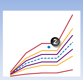
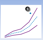
Example
The example depicted below demonstrates a breach of the secondary deviation limit, causing a secondary event to occur.
- Input mode is values.
- Deviation mode is a percentage value.
- Curve settings are X-Y values; that is, they are static.
- The sample interval is every two hours.
 |
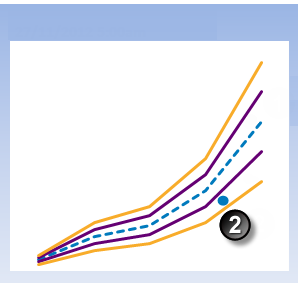 |
 |
Duration Limit
Monitor for data that continuously exceeds the primary deviation limit, for longer than the secondary state duration limit.
If data that continuously exceeds the primary deviation limit for longer than specified in the secondary state duration limit, a secondary event occurs, and a secondary state is reached.
Example
- Input mode is values.
- Deviation mode is a percentage value.
- Secondary state duration is set to 5 hours.
- Curve settings are X-Y values; that is, they are static.
- The sample interval is every two hours.
| Duration and Limits | Duration of data continuously exceeding the primary deviation limit | |||
|---|---|---|---|---|
 |
 |
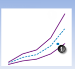
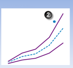
At 1:00am, primary state duration is at zero. | ||
 |
 |
At 3:00am, primary state duration is at zero. The primary limit has been exceeded, so timing of primary duration starts now. | ||
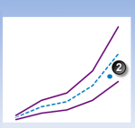
 |
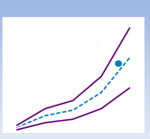
At 5:00am, the X and Y coordinates of the data place it below the lower primary deviation limit. The primary state endures. |  |
At 5:00am, primary state duration is now at 2 hours (a full sample interval). | |
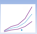
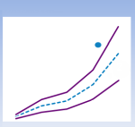
 |
At 7:00am, the X and Y coordinates of the data place it below the lower primary deviation limit. The primary state endures. |  |
At 7:00am, primary state duration is now at 4 hours (two full sample intervals). | |
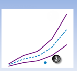
 |
At 9:00am, the X and Y coordinates of the data place it above the upper primary deviation limit. The primary state endures. |  |
||
Sustained Value Limit
Monitor for when data exceeds the primary deviation limit for more than a specified number of times (secondary state, sustained value limit), consecutively. If this is the case, a secondary event occurs and a secondary state is reached.
Example
- Input mode is values.
- Deviation mode is a percentage value.
- Secondary state sustained value limit is set to 3.
- Curve settings are X-Y values; that is, they are static.
- The sample interval is every two hours.
| Duration and Limits | |||
|---|---|---|---|
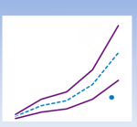
|
|
|
|
At 1:00am, the primary deviation limit has been exceeded zero times. |
|
|
|
|
At 3:00am, the primary deviation limit has been exceeded once. |
|
|
At 5:00am, the X and Y coordinates of the data place it below the lower primary deviation limit. The primary state endures. |
|
At 5:00am, the primary deviation limit has been exceeded twice (consecutively). |
|
|
At 7:00am, the X and Y coordinates of the data place it below the lower primary deviation limit. The primary state endures. |
|
At 7:00am, the primary deviation limit has been exceeded three times (consecutively). |
|
|
At 9:00am, the X and Y coordinates of the data place it above the upper primary deviation limit. The primary state endures. |
|
|


Rolling Sum Total Duration Limit
Monitor for a specified accumulated duration of all periods where data is in breach of the primary deviation limit, within the preceding specified secondary state rolling sum period.
If the total combined primary state duration is longer than the specified secondary state rolling sum duration limit, a secondary event occurs, and a secondary state is reached.
Example
- Input mode is values.
- Deviation mode is a percentage value.
- Secondary state duration is set at 5 hours.
- Curve settings are X-Y values; that is, they are static.
- The sample interval is every two hours.
|
Duration and Limits |
Accumulated duration of data exceeding the primary deviation limit |
|||
|
|
|
|
At 1:00am, duration is at zero. Primary limit has been exceeded, so timing starts now. |
|
|
|
|
|
At 3:00am, the accumulated duration is now at 2 hours (a full sample interval). The process is no longer in the primary state, so timing stops. |
|
|
|
|
|
At 5:00am, the accumulated duration remains at 2 hours (a single sample interval). The primary limit has been exceeded, so timing starts again. |
|
|
|
At 7:00am, the X and Y coordinates of the data place it above the upper primary deviation limit. |
|
At 7:00am, the accumulated duration is now at 4 hours (two full sample intervals). The process is still in the primary state, so timing continues. |
|
|
|
At 9:00am, the X and Y coordinates of the data place it above the upper primary deviation limit. |
|
|
|


Rolling Sum Breach Occurrences Limit
Monitor for when a set number of values (secondary state breach occurrences limit) has breached the primary deviation limit, during the preceding specified secondary rolling sum period.
Example
In the following example, the secondary state breach occurrences limit is set to 2.
- Input mode is values.
- Deviation mode is a percentage value.
- Secondary state rolling sum breach occurrences limit is set at 2.
- Curve settings are X-Y values; that is, they are static.
- The sample interval is every two hours.
| Duration and Limits | Accumulated Breach Occurrences | |||
 |
|
|
At 1:00am, breach occurrences counter is one. |
|
|
|
|
|
At 3:00am, breach occurrences counter remains at one. |
|
|
|
At 5:00am, the X and Y coordinates of the data place it between the upper and lower primary deviation limits. The default state endures. |
|
At 5:00am, breach occurrences counter remains at one. |
|
|
|
|
|
|
|


Tertiary State
There are several ways to reach the tertiary state outcome in the Performance Curve process:
- Deviation Limit
- Duration Limit
- Sustained Value Limit
- Rolling Sum Total Duration Limit
- Rolling Sum Breach Occurrences Limit
You can choose to set one or more conditions to trigger the tertiary state. For example, a test may have a tertiary deviation limit defined, as well as configured variables for determining tertiary state rolling sum breach occurrences.
Deviation Limit
If the configured tertiary deviation limit is breached, a tertiary event occurs, and a tertiary state is reached.
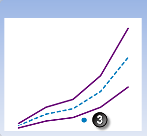
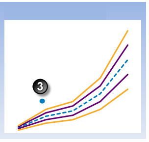
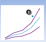
The graph demonstrates a breach of the tertiary deviation limit, causing a tertiary event to occur.
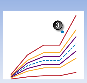
Example
The example depicted below demonstrates a breach of the tertiary deviation limit, causing a tertiary event to occur.
- Input mode is values.
- Deviation mode is a percentage value.
- Curve settings are X-Y values; that is, they are static.
- The sample interval is every two hours.
Data item |
Expected curve |
Primary deviation limit |
Secondary deviation limit |
Tertiary deviation limit |
| 5:00am | 7:00am | 9:00am |
 |
 |
 |
Duration Limit
Monitor for data that continuously exceeds the primary deviation limit, for longer than the tertiary state duration limit.
If data that continuously exceeds the primary deviation limit for longer than specified in the tertiary state duration limit, a tertiary event occurs, and a tertiary state is reached.
Example
- Input mode is values.
- Deviation mode is a percentage value.
- Curve settings are X-Y values; that is, they are static.
- The sample interval is every two hours.
- Secondary state duration is set at 1.5 hours.
- Tertiary state duration is set at 3.5 hours.
Data item |
Expected curve |
Primary deviation limit |
Primary state duration |
Start of primary state |
Current time |
| Duration and Limits | Duration of data continuously exceeding the primary deviation limit | |||
|---|---|---|---|---|
 |
 |
At 1:00am, duration is at zero. | ||
 |
 |
At 3:00am, duration is at zero. Primary limit has been exceeded, so timing starts now. | ||
 |
At 5:00am, the X and Y coordinates of the data place it below the lower primary deviation limit. The primary state endures. |  |
At 5:00am, duration is now at 2 hours (a full sample interval), exceeding the secondary state duration limit of 1.5 hours. A secondary state is reached, and a secondary event is raised. | |
 |
At 7:00am, the X and Y coordinates of the data place it below the lower primary deviation limit. The secondary state endures. |  |
||
Sustained Value Limit
Monitor for when data exceeds the primary deviation limit for more than a specified number of times (tertiary state sustained value limit), consecutively. If this is the case, a tertiary event occurs, and a tertiary state is reached.
Example
- Input mode is values.
- Deviation mode is a percentage value.
- Curve settings are X-Y values; that is, they are static.
- The sample interval is every two hours.
- Secondary state sustained value limit is set at 2.
- Tertiary state sustained value limit is set at 3.
Data item |
Expected curve |
Primary deviation limit |
Primary state duration |
Start of primary state |
Occurrence counter |
| Duration and Limits | |||
|---|---|---|---|
 |
At 1:00am, the primary deviation limit has been exceeded zero times. | ||
 |
At 3:00am, the primary deviation limit has been exceeded once. | ||
 |
At 5:00am, the X and Y coordinates of the data place it below the lower primary deviation limit. | ||
 |
At 7:00am, the X and Y coordinates of the data place it beyond the primary deviation limit. |
Rolling Sum Total Duration Limit
Monitor for a specified accumulated duration of all periods where data is in breach of the primary deviation limit, within the preceding specified tertiary state rolling sum period.
If the total combined primary state duration is longer than the specified tertiary state rolling sum duration limit, a tertiary event occurs, and a tertiary state is reached.
Example
- Input mode is values.
- Deviation mode is a percentage value.
- Curve settings are X-Y values; that is, they are static.
- The sample interval is every two hours.
- Secondary state duration is set at 3.5 hours.
- Tertiary state duration is set at 5 hours.
Start of primary state |
Primary deviation limit |
Exceeding primary limits |
Current rolling sum period |
| Duration and Limits | Accumulated duration of data exceeding the primary deviation limit | |||
|---|---|---|---|---|
|
|
|
 |
At 1:00am, duration is at zero. Primary limit has been exceeded, so timing starts now. | |
 |
 |
At 3:00am, the accumulated duration is now at 2 hours (a full sample interval). Input data is no longer exceeding the primary limits, so timing stops. | ||
 |
 |
At 5:00am, the accumulated duration remains at 2 hours (a single sample interval). Input data is beyond primary limits, so timing resumes. | ||
 |
At 7:00am, the X and Y coordinates of the data place it of the data place it above the upper primary deviation limit. |  |
||
 |
At 9:00am, the X and Y coordinates of the data place it above the upper primary deviation limit. |  |
||
Rolling Sum Breach Occurrences Limit
Monitor whether a set number of values (tertiary state breach occurrences limit) has breached the primary deviation limit, during the preceding specified tertiary rolling sum period. If this occurs, a tertiary event is raised, and a tertiary state is reached.
Example
In the following example, the tertiary state rolling sum breach occurrences limit is set to 3.
- Input mode is values.
- Deviation mode is a percentage value.
- Curve settings are X-Y values; that is, they are static.
- The sample interval is every two hours.
- Secondary state rolling sum breach occurrences limit is set to 2.
- Tertiary state rolling sum breach occurrences limit is set to 3.
Start of primary state |
Primary deviation limit |
Primary state duration |
Current rolling sum period |
Occurrence counter |
| Duration and Limits | Accumulated Breach Occurrences | |||
 |
 |
At 1:00am, breach occurrences counter is one. | ||
 |
 |
At 3:00am, breach occurrences counter remains at one. | ||
 |
 |
|||
 |
At 7:00am, the X and Y coordinates of the data the X and Y coordinates of the data place it above the upper primary deviation limit. | 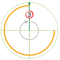 |
||
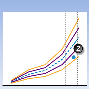
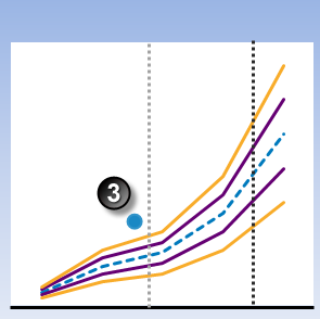
Out of Range State
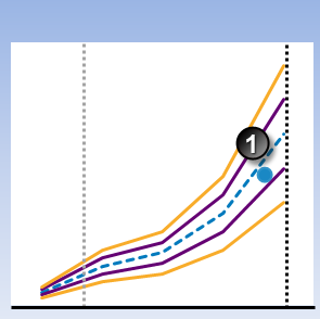
If the X coordinate of the data is outside the range defined by Min X and Max X, an out of range event occurs, and an out of range state is reached.
Example
In the following example, Min X and Max X are both fixed values.
- Input mode is values.
- Deviation mode is a percentage value.
- Curve settings are X-Y values; that is, they are static.
- The sample interval is every two hours.
- Secondary state rolling sum breach occurrences limit is set to 2.
- Min X and Max X are both fixed values.
Data item |
Expected curve |
Primary deviation limit |
Secondary deviation limit |
X Axis |
Min X |
Max X |
| 5:00am | 7:00am | 9:00am |
 |
 |
 |
A default state is reached, and a default event is raised. |
At 9:00am, the X and Y coordinates of the data place it above the upper secondary deviation limit. This would normally cause a secondary event. | |
| Evaluate whether the X coordinate is within the range. | ||
| In addition, the X coordinate is within the range defined by Min X and Max X. | In addition, the X coordinate is within the range defined by Min X and Max X. | |
Adding a Performance Curve Process
The Performance Curve Process compares process variable data against defined limits and conditions. If a limit or condition is breached when the process is executed, a new state is reached and an event is raised.
Setting Process Values and Limits
Part of setting up the Performance Curve process involves selecting limits, such as the primary state deviation limit, secondary state deviation limit, tertiary state deviation limit, breach occurrences limits and so on. Limits can either be fixed values, or they can be variable data taken from entities.
The following limits are available. Select a limit type from the drop-down list, then type in or select a limit.
- Fixed Value: Type in a numerical value.
- Attribute: This option is only available if the test’s Source Type is Entity or Hierarchy. Click the ellipsis
 button to select an attribute of the source entities.
 - Source Tag: This option is only available if the Source Type is Tag.
- Calculation: Click the ellipsis
 button to open the Edit Calculation window.
- If the Source Type is Entity or Hierarchy: Type a calculation, prefixed by ‘this’ as the Source Entity token, for example: {this:THP} + 34.
- If the Source Type is Tag: Type a calculation, prefixed by ‘this’ as the Source Tag token, for example: {this} * 2.
- Tag: Click the ellipsis
 button to select a tag.
 - Entity Attribute: Click the ellipsis
 button to select an entity. From here, select an attribute, or attribute value, for the selected entity.
Adding the Process
As with all Sentinel processes, the Performance Curve Process is defined within a Sentinel Test page. In the Sentinel Test page:
1. Expand the Process ![]() panel.
panel.
2. Select Performance Curve from the Process drop-down list.
A. Input Settings
There are two input modes available to the Performance Curve process:
- Values
- Liquid Control Valve
Values
- Select Values from the Input Mode drop-down list.
- Specify the X and Y coordinates, which are used for creating the curves. For each coordinate, select one of the following from the drop-down list; then type in or select a corresponding value:
-
- Fixed Value
- Attribute (only available if the Source Type is Entity or Hierarchy)
- Source Tag (only available if the Source Type is Tag)
- Calculation
- Tag
- Entity Attribute
Liquid Control Valve
- Select Liquid Control Valve from the Input Mode drop-down list.
- Specify the X and Y coordinates, which are used for creating the curves.
- For the X coordinate, select one of the following from the drop-down list; then type in or select a corresponding value:
-
-
- Fixed Value
- Attribute (only available if the Source Type is Entity or Hierarchy)
- Source Tag (only available if the Source Type is Tag)
- Calculation
- Tag
- Entity Attribute
- For the Y coordinate, there are three factors:
- Flow Rate (US gallons per minute)
- Specific Gravity
- Pressure Drop
-
For each of these, select one of the following from the drop-down list; then type in or select a corresponding value:
-
-
- Fixed Value
- Attribute (only available if the Source Type is Entity or Hierarchy)
- Source Tag (only available if the Source Type is Tag)
- Calculation
- Tag
- Entity Attribute
-
B. Curve Settings
The curve settings determine how the curve is created, using the input settings as a base factor. There are two types of curve to choose from:
- Polynomial
- X-Y Values
X-Y Values
Points are plotted directly from the X and Y coordinates as they are captured into the table. The resulting graph forms the basis of the Performance Curve limits. The recommended maximum number of X-Y pairs is 10.
- From the Curve Type drop-down list, select X-Y Values.
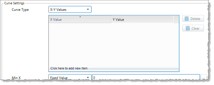
- Add the X and Y values.
- Click Click here to add new item, located at the end of the table.

This is replaced with two text boxes: one each for the X and Y values, with the cursor positioned in the first box.

- Capture the X value in the left text box (the X Value box), then press the tab key to move the cursor to the second text box (the Y Value box).

- Capture the Y value.

- Press the Tab key.
The X and Y values are added to the table, and Click here to add new item reappears to replace the two text boxes.
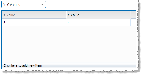
- Click Click here to add new item, located at the end of the table.
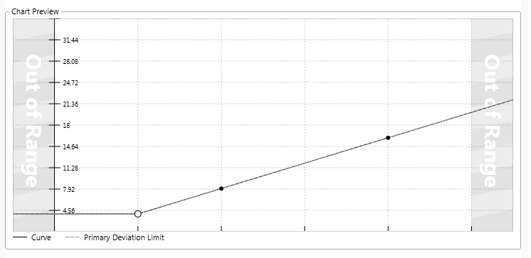
- Add the second pair of X and Y values.
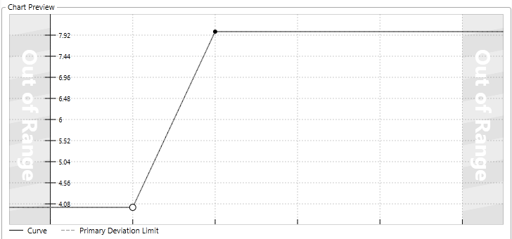
The Chart Preview (located below the Curve Settings section) now has a line drawn between the first two pairs of coordinates:
- Continue to add X and Y values in this way, until your table of X-Y values is captured.

Each pair of values is added to the table in numerical order of the X value.
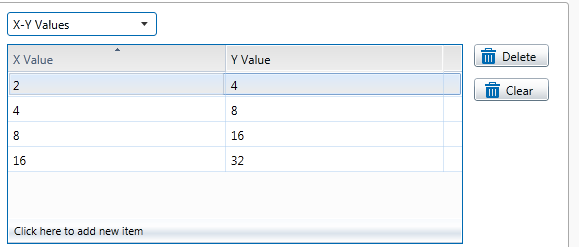
The Chart Preview now displays the line connecting all of the coordinate pairs:
Update a Pair of X-Y Values
- Select the pair that you want to update by clicking the mouse on the row (or select the row by selecting the corresponding point on the chart).
- To update the X value, click in the X Value table item; then overtype with a new value.
- To update the Y value, click in the Y Value table item; then overtype with a new value.
Delete an X-Y Pair from the Table
- Select the pair that you want to delete by clicking the mouse on the row (or select the row by selecting the corresponding point on the chart).
- Click the Delete button to the right of the table.
The row is removed from the table, and the Chart Preview adjusts to reflect this.
Clear All X-Y Values in the Table
- Click the Clear button to the right of the table.
All rows are removed from the table, and the Chart Preview is cleared.
Using the Chart to Select a Row on the Table
- If you want to change the values for a particular point on the chart, click that point.
The solid point on the chart changes to a circle, and the cursor highlights the corresponding row on the table of X-Y values. - You can then update these values in the row.
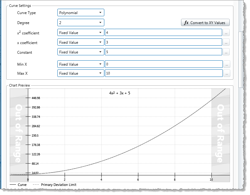
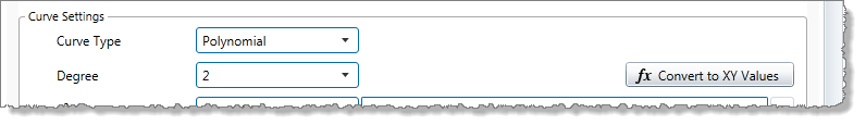
Polynomial curve
Points are plotted using values derived from the polynomial equation. The resulting graph forms the basis of the Performance Curve limits. There are up to 9 degrees of polynomial.
1. From the Curve Type drop-down list, select Polynomial (the default).
2. Select the number of degrees for the polynomial equation, from the Degrees drop-down list. The default is 2.
3. Select the different factors for the equation. Each of these values may be any of the following:
- Fixed Value
- Attribute (only available if the Source Type is Entity or Hierarchy)
- Source Tag (only available if the Source Type is Tag)
- Calculation
- Tag
- Entity Attribute
The number of coefficients to capture depends on the polynomial degree selected.
Note: When capturing fixed values, you may use negatives. Decimal values are rounded up to the second place.
4. Capture the highest coefficient. For a 5th degree polynomial, this is the x5 coefficient. For a 3rd degree polynomial, this is the x3 coefficient, and so on.
5. Capture the next highest coefficient (for a 5th degree polynomial, this is the x4 coefficient).
6. Continue until all coefficients have been captured, including the x coefficient.
7. Capture the constant value in the Constant text box.
The chart resulting from these factors is displayed in the Chart Preview below:
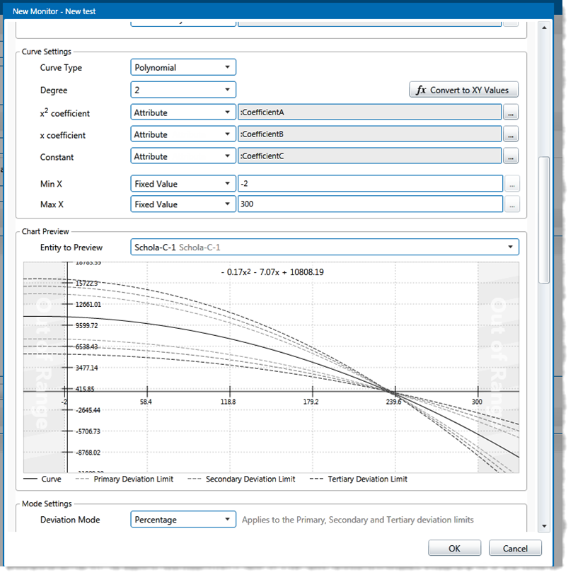
Selecting the Entity to Preview
If the process is using a hierarchy as the source and an entity (attribute or entity) in the curve settings, you can select which entity to preview in the chart. The entities listed are those that belong to the selected hierarchy.
- Select an entity from the Entity to Preview drop-down list.
The current values of the entities of the selected coefficients are applied to the equation. This is reflected in the chart preview.
Converting to X-Y Values
If you want to adjust the polynomial curve, you can use the Convert to XY Values function.
1. Click the fx Convert to XY Values button.
A Convert to XY Values window appears.
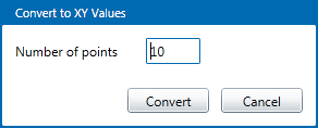
2. Select the number of points, by typing a positive integer in the Number of points box, then click Convert.
The Curve Settings are converted to XY Values, and the resulting chart is now made up of lines connecting the coordinate pairs.
In this example 5 points were selected.
3. Adjust any of these points to refine the chart, if necessary (see “Defining X-Y Values” above).
Out of Range Values
A range of acceptable values is defined by a Min X and a Max X value. The default range is 0: 10 (defined by Min X : Max X).
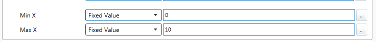
To change the range, select one of the following from the drop-down list, and then type in or select a corresponding value, for both Min X and Max X:
- Fixed Value
- Attribute (only available if the Source Type is Entity or Hierarchy)
- Source Tag (only available if the Source Type is Tag)
- Calculation
- Tag
- Entity Attribute
If fixed values are used, the Out of Range values cause an adjustment to the Chart Preview.
C. Mode Settings
Define whether the deviation mode is a percentage or an absolute value, to establish how primary, secondary and tertiary deviation limits are calculated. Also select whether to set upper or lower deviation limits, or both.
Note: The mode settings apply to primary, secondary and tertiary deviation limits.
- From the Deviation Mode drop-down list, select Percentage or Absolute Value.
The deviation mode determines how the deviation limits will be calculated. - Select the Upper Deviation check box to set an upper deviation limit.
- Select the Lower Deviation check box to set a lower deviation limit.
D. Deviation Limits
Note: The Primary Deviation Limit is mandatory for the Performance Curve Process.
1. From the Primary Limit drop-down list, select one of the following and then type in or select a corresponding value:
- Fixed Value
- Attribute (only available if the Source Type is Entity or Hierarchy)
- Source Tag (only available if the Source Type is Tag)
- Calculation
- Tag
- Entity Attribute
2. Optionally define secondary limits in the same way (first select the Secondary Limit check box).
3. Optionally define tertiary limits in the same way (first select the Tertiary Limit check box).
The Chart Preview changes to show how the limits are applied.
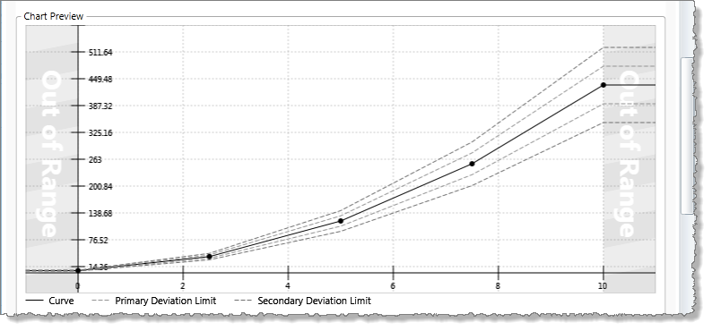
The chart above shows primary and secondary upper and lower deviation limits of fixed values 10 and 20 respectively. Here, limits are calculated using the percentage deviation mode.
Using the same settings but applying the absolute value mode, deviation limits are calculated differently, as shown in the following chart preview:
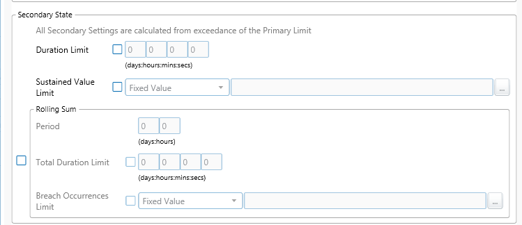
E. Secondary State
Note: All Secondary State settings are calculated from the primary deviation limit.
All secondary state settings are captured or selected in the Secondary State section of the process, with the exception of the Secondary Deviation Limit, which is set in the Deviation Limit Settings section of the process.
Duration Limit
The Secondary State Duration Limit is used for monitoring where data is continuously beyond the primary deviation limit, for longer than the specified secondary duration limit.
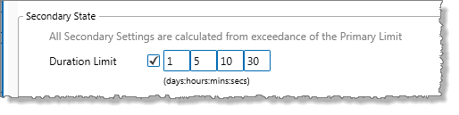
In the Secondary State section:
- Select the Duration Limit check box.
- Type integer values in the days, hours, mins (minutes), and secs (seconds) Duration Limit boxes to define a duration period. The default value is zero.
Sustained Value Limit
The Secondary State Sustained Value Limit is used for monitoring where data is beyond the primary deviation limit for more than a specified number of times (secondary state sustained value limit), consecutively.
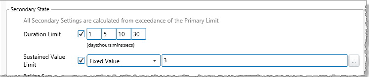
In the Secondary State section:
1. Select the Sustained Value Limit check box.
2. From the Sustained Value Limit drop-down list, select one of the following and then type in or select a corresponding value:
- Fixed Value
- Attribute (only available if the Source Type is Entity or Hierarchy)
- Source Tag (only available if the Source Type is Tag)
- Calculation
- Tag
- Entity Attribute
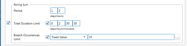
Rolling Sum Period
The rolling sum period is a defined period (specified in days and hours). At every sample interval, the rolling sum period applies to that period preceding the sample interval.
Set a secondary state rolling sum period if you are going to define a secondary state total duration limit or a secondary state breach occurrences limit.
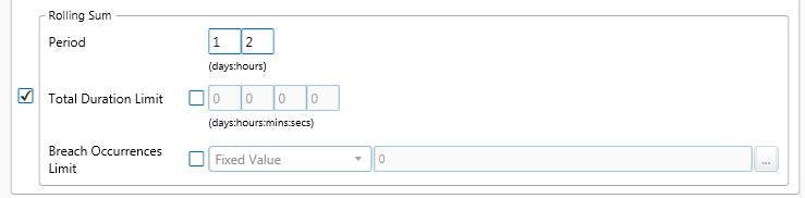
In the Secondary State section:
1. Select the check box to the left of the Rolling Sum section.
2. Type integer values in the days and hours Period boxes to define the rolling sum period. The default value is zero.
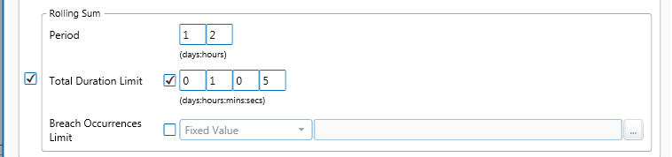
Rolling Sum Total Duration Limit
The Secondary State Rolling Sum Total Duration Limit is used to monitor for a specified accumulated duration of all periods where data is in breach of the primary deviation limit, within the preceding specified secondary state rolling sum period.
1. In the Rolling Sum section, within the Secondary State section:
2. Select the Total Duration Limit check box.
3. Type integer values in the days, hours, mins (minutes), and secs (seconds) Total Duration Limit boxes to define a total duration limit period. The default value is zero.
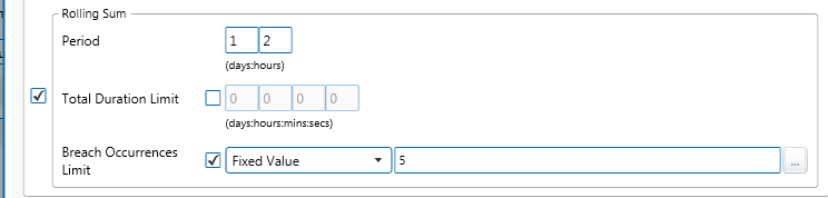
Rolling Sum Breach Occurrences Limit
The Secondary State Rolling Sum Breach Occurrences Limit is used to monitor for when a set number of values (secondary state breach occurrences limit) has breached the primary deviation limit, during the preceding specified secondary state rolling sum period.
In the Rolling Sum section, within the Secondary State section:
1. Select the Breach Occurrences Limit check box.
2. From the Breach Occurrences Limit drop-down list, select one of the following and then type in or select a corresponding value:
- Fixed Value
- Attribute (only available if the Source Type is Entity or Hierarchy)
- Source Tag (only available if the Source Type is Tag)
- Calculation
- Tag
- Entity Attribute
F. Tertiary State
Note: All Tertiary State settings are calculated from the primary deviation limit.
All tertiary state settings are captured or selected in the Tertiary State section of the process, with the exception of the Tertiary Deviation Limit, which is set in the Deviation Limit Settings section of the process.
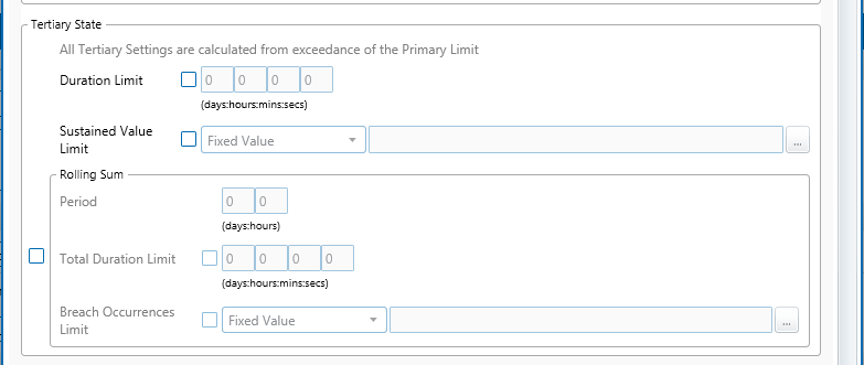
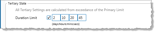
Duration Limit
The Tertiary State Duration Limit is used for monitoring where data is continuously beyond the primary deviation limit, for longer than the specified tertiary state duration limit.
In the Tertiary State section:
1. Select the Duration Limit check box.
2. Type integer values in the days, hours, mins (minutes), and secs (seconds) Duration Limit boxes to define a duration period. The default value is zero.
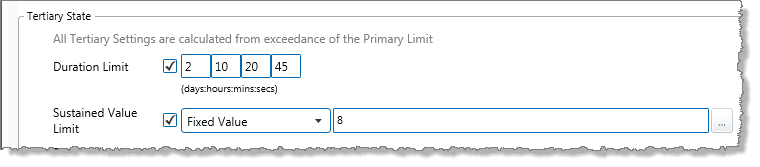
Sustained Value Limit
The Tertiary State Sustained Value Limit is used for monitoring where data is beyond the primary deviation limit for more than a specified number of times (tertiary state sustained value limit), consecutively.
In the Tertiary State section:
1. Select the Sustained Value Limit check box.
2. From the Sustained Value Limit drop-down list, select one of the following and then type in or select a corresponding value:
- Fixed Value
- Attribute (only available if the Source Type is Entity or Hierarchy)
- Source Tag (only available if the Source Type is Tag)
- Calculation
- Tag
- Entity Attribute
These different options are outlined above, in the section: “Setting Process Values and Limits”, above.
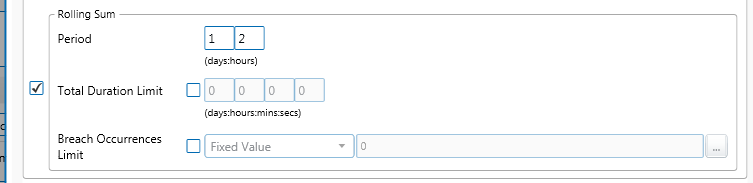
Rolling Sum Period
The rolling sum period is a defined period (specified in days and hours). At every sample interval, the rolling sum period applies to that period preceding the sample interval.
Set a tertiary state rolling sum period if you are going to define a Tertiary State Total Duration Limit or a Tertiary State Breach Occurrences Limit.
In the Tertiary State section:
1. Select the check box to the left of the Rolling Sum section.
2. Type integer values in the days and hours Period boxes to define the rolling sum period. The default value is zero.
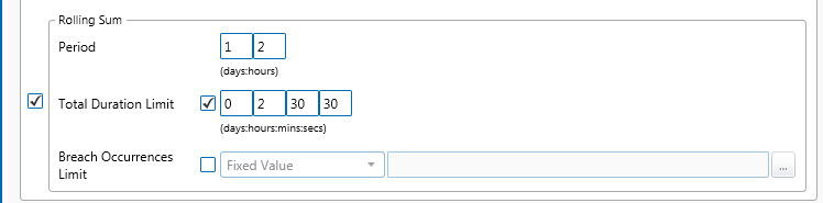
Rolling Sum Total Duration Limit
The Tertiary State Rolling Sum Total Duration Limit is used to monitor for a specified accumulated duration of all periods where data is in breach of the primary deviation limit, within the preceding specified tertiary state rolling sum period.
In the Rolling Sum section, within the Tertiary State section:
1. Select the Total Duration Limit check box.
2. Type integer values in the days, hours, mins (minutes), and secs (seconds) Total Duration Limit boxes to define a total duration limit period. The default value is zero.
Rolling Sum Breach Occurrences Limit
The Tertiary State Rolling Sum Breach Occurrences Limit is used to monitor for when a set number of values (tertiary state breach occurrences limit) has breached the primary deviation limit, during the preceding specified tertiary rolling sum period.
In the Rolling Sum section, within the Tertiary State section:
1. Select the Breach Occurrences Limit check box.
2. From the Breach Occurrences Limit drop-down list, select one of the following and then type in or select a corresponding value:
- Fixed Value
- Attribute (only available if the Source Type is Entity or Hierarchy)
- Source Tag (only available if the Source Type is Tag)
- Calculation
- Tag
- Entity Attribute
G. Adding Comments
- To add comments to the process panel click the comment
 button, at the top right of the panel.
Configuring States
For the Performance Curve process, you can configure the following states, each with an optional state override and comments:
- Primary
- Secondary
- Tertiary
- Out of Range
- Suppressed
You cannot change the severity of the Default state; however, you can add a state override and comments.
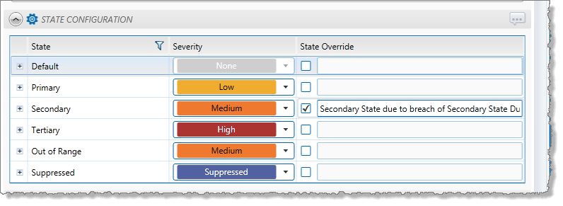
Note: Only configure states where you have set a limit.