ON THIS PAGE:
In IFS OI Server, data may be requested raw or processed in some way. Currently the three kinds of data processing available are average, last known value, and linear interpolate. In IFS OI Server these different aggregations are known as sample methods.
How each of these sample methods is determined can vary from one source of data to another. Most Historians already have these functions built in, so IFS OI Server delegates these aggregations to the Historian to perform, so that we get the fastest and most accurate aggregations possible.
For any systems that do not have such features, IFS OI Server has a built-in set that will be used. This article describes how these functions process the data.
Background
Before we get into how these methods work, let’s define some of the other inputs to these functions. When we ask IFS OI Server for data we need to specify a few parameters so that IFS OI Server knows what to do with the data.
|
Start and End time (Request Interval) |
The start and end time for the request is sometimes called the request interval. These two times specify the whole range over which we want data. Note that start and end times are inclusive. For example, if we want data for the whole day, we may use 1/1/2015 00:00 and the 1/1/2015 23:59 to specify that we want data for that day only. Note that the calling application (e.g. IFS OI Explorer) must send the request interval to IFS OI Server in UTC. When getting data from IFS OI Server, depending on how you set the request interval, you can get IFS OI Server to return different numbers of results. These two different methods are known as Range Fetches and Single Point (or Spot) Fetches. |
|
Sample Interval (Density) |
The sample interval is the amount of time between each data point that will be returned. If we set the sample interval to 3600 seconds, we will get a data point returned every hour between the start and end time (request interval). If that start and end time are 1 day apart, we will get 24 values returned, one per hour. |
|
Sample Methods |
The rest of this article details how the built-in aggregations work inside IFS OI Server. Note that if the source system natively supports any of the following sample methods, adaptors will often be written to use the source system’s functions, rather than IFS OI Server’s calculations as described below. However this is dependent on the adaptor itself. |
Formulas
Average
The Average sample method returns a time-weighted average of the raw data for each sample interval over the specified request interval. The set of time-value pairs returned are generated using the following formula:
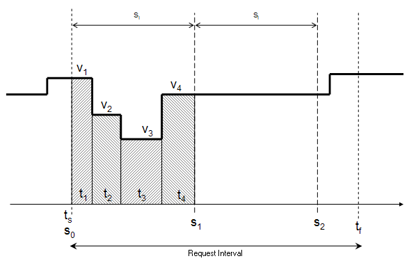
The request interval [ts, tf] is divided into intervals using the configured sample interval SI. If the specified request interval is not an integral multiple of SI, then the returned results will cover slightly less than the desired interval (this gap is the interval [S2, tf].
As a result, the request interval [ts, tf] will be broken into N intervals, where:
![]()
There will be N aggregate values returned at times (s0, s1, … , sN), where:
![]()
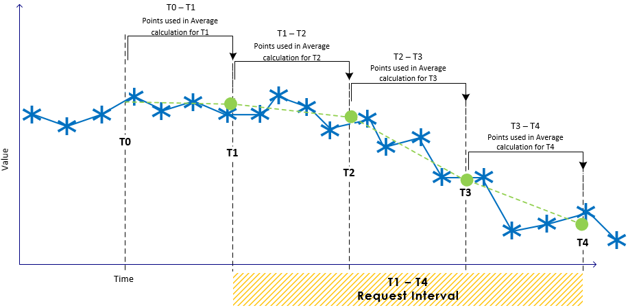
A time-weighted average is calculated for each interval, which factors into the result the amount of time each raw value was held during the sample interval.
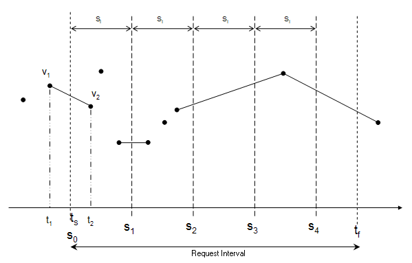
In the above figure, the result for the second interval (s1,s2) will be v4, since the value is constant over the entire interval. As the raw value changes during (s0,s1), the reported value will be an average of the four raw values over that interval, weighted by the duration that each raw value is held:
The data used to calculate an average value for s0 is based on an interval of SI that ends at s0. To fulfil a request for average-sampled data at a particular instant in time (ti), the adaptor examines the raw data over the interval (ti-SI, ti) and calculates the time-weighted average value over that interval. The value is reported for time ti.
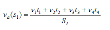
Last Known Value
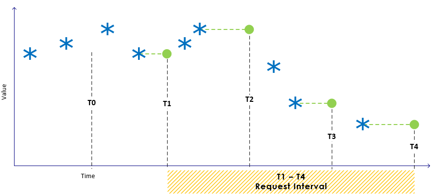
The calculations of last known value data returns the last known raw value at the end of each sampling interval. As with time-weighted average data, the request interval [ts,tf] is first divided into N sample intervals, and values are reported for the end of each interval. The set of reported values are simply the raw value of the input at each of the times (s0, s1, … , sN).
In the above figure, the returned data would be three points: (s0,v1), (s1,v4) and (s2,v4). For last-known-value at a single-point instant, the algorithm looks for the most recent raw value from the source, but returns it with a timestamp of the requested sample interval time, which will be the same or after the raw value's actual time (the time of s0, S1 and S2).
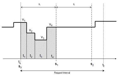
Linear Interpolate
For linear interpolate aggregate data, the sample period (ts, tf) is divided into intervals using the same process as for time-weighted average and last known value.
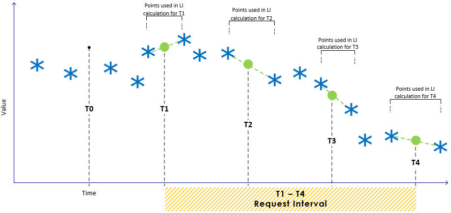
Sample values are reported at the start of the request period, and all sample interval boundaries: (s0, s1, …, sN). For each sample point, the formula looks for the most recent raw value and the closest subsequent raw value, and uses those two values as end points of a line. The value of that line at the sample point is the returned aggregate value.
In the above figure, the value at s0 is based on the nearest previous value at t1 and the nearest subsequent value at t2. The value reported at s0 would be:
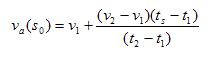
In some situations, such as the values for s2 and s3, the same two raw value data points may be used to calculate linear interpolated values for two different sample points. For the last sample point, the formula will need a raw value potentially beyond the end of the requested sample period (after tf). The adaptor looks forward in time using configuration values to find the next raw value.
Adaptive Raw
The Adaptive Raw sample method allows a very close approximation of raw data to be displayed by consuming applications, such as the Explorer Trend, at a much faster rate than was previously possible using raw data.
When analyzing data in fine detail, we often want to get the most granular data possible onto the trend. Traditionally, using the Raw sample method we could end up with millions of points of data being returned, with no way of actually showing all of these points on a screen with a resolution of 1920 pixels. Transferring all of those data points back to the web browser would also take a long time.
Adaptive Raw is a new algorithm implemented in IFS OI Server’s calculation engine that is designed to provide the best of both worlds: a trace on the Trend that is virtually identical in appearance, but is much, much faster. When using Adaptive Raw, IFS OI Server does the work of automatically selecting the sample interval to return the most detailed data possible.
The Adaptive Raw sample method works by sending all Raw data points from the historian to IFS OI Server, and then determining the number of points. If there are less than 2000 points then the raw data is returned, otherwise the adaptive raw algorithm is used to return 2000 points. Essentially, the Adaptive Raw sample method chooses the best data for you. The processing returns a trace that is a very accurate representation of a traditional Raw trend, but with far less data being actually transferred to the trend.
Using this method, we have been able to open up the time ranges available for trending of data using Adaptive Raw, giving an almost perfect copy of a raw Trend, but at a vastly faster speed.
Cheat Sheet
The following images provide a simplified overview of how the sample methods are calculated.
|
Linear Interpolate:
|
Average:
|
|
Last Known Value:
|
|
Release History
- Data Transformation and Sample Methods 4.5.4 (this release)
- Added Adaptive Raw sample method
- Data Transformation and Sample Methods 4.3.0
- Initial release