Contents
When getting data from P2 Server, depending on how you set the request interval, you can get P2 Server to return different numbers of results. These two different methods are known as Range Fetches and Single Point (or Spot) Fetches.
Range Fetch
A Range Fetch is one where the start time and end time are set to different values, and a stream of data is returned. An example of this may be setting the start time as 1-1-2015 and the end time as 2-1-2015. Range fetches like this will return 1 or more data points, depending on the sample interval and the presence of data in the source system.
The P2 Explorer trend is an example of where a range fetch is used, as we want a continuous stream of data being returned for the time period chosen. In the following example, the source system has data for the specified time period. If there is no data for that period, no data points would be returned.
For Average, Last Known Value, and Linear Interpolate sample methods, the first result returned should be at the Start Time, with subsequent values at each sample interval forwards from that time, up to and including the End Time. If the duration between the Start Time and End Time is not a whole number of intervals, then no value is returned at the End Time.
For the Raw sample method, the sample interval has no effect.
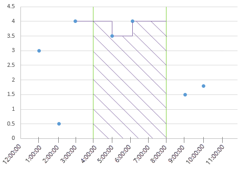
Ranged Raw
Ranged Raw sampling returns all values, and their timestamps, that occur between and including the Start Time and End Time, if they exist. In this scenario, a request is made for the ranged raw values between a Start Time of 2:00:00 AM and an End Time of 8:00:00 AM.
Parameters: Start Time = 2:00:00 AM, End Time = 8:00:00 AM
Return values:
Value = 0.5, Timestamp = 2:00:00 AM
Value = 4, Timestamp = 3:00:00 AM
Value = 3.5, Timestamp = 5:00:00 AM
Value = 4, Timestamp = 6:00:00 AM
No value is returned for the End Time, as none exists.
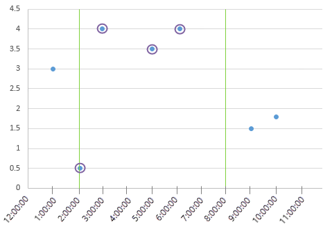
Ranged Last Known Value
This method returns a series of values determined via the Last Known Value method, spaced regularly between the start and end time according to the Interval parameter.
As with Single Point Last Known Value, the returned timestamps are based on the request time (in this case the request / interval times), and not the raw timestamp of the underlying data.
A ranged last known value sampling is requested with a Start Time of 2:00:00 AM, an End Time of 8:00:00 AM, and an Interval of 9000 seconds (2.5 hours).
- The value 0.5 exists at 2:00:00 AM, so this value is returned with a timestamp of 2:00:00 AM.
- The next interval is at 4:30:00 AM, and because no value exists here, the last occurring value of 4 is extrapolated to this point and returned with the 4:30:00 AM timestamp.
- The same process is applied for the 7:00:00 AM interval, where the value 4 is extrapolated and returned with the timestamp of 7:00:00 AM.
- The next interval exceeds the parameter of our end time, so no value is returned here. End Time values are only returned if the End Time is an integer multiple of intervals after the Start Time, that is, where the Interval and the End Time line up.
Parameters: Start Time = 2:00:00 AM, End Time = 8:00:00 AM, Interval = 9000 seconds
Return values:
Value = 0.5, Timestamp = 2:00:00 AM
Value = 4, Timestamp = 4:30:00 AM
Value = 4, Timestamp = 7:00:00 AM
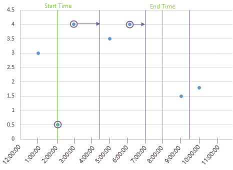
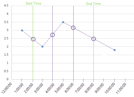
Ranged Linear Interpolate
This method returns a series of values determined via the Linear Interpolate method, spaced regularly according to the Interval parameter, between the Start Time and End Time.
As with Single Point Linear Interpolate, each value is calculated using a gradient between the first value occurring before and the first value occurring after the respective request time / interval time, with the return value being the intersect of the gradient with the request time / interval time. These values are returned with their respective timestamps, which are based on the request time / interval time.
A Ranged Linear Interpolate sampling is requested with a Start Time of 2:00:00 AM, an End Time of 8:00:00 AM, with an Interval of 7200 seconds (2 hours).
- Data at the Start Time interval does not exist, so the linear interpolate is calculated between the last occurring value before the interval and the first occurring value after the interval, which are 3 and 2 respectively.
- The linear interpolate at 4:00:00 AM is calculated using the raw values at 3:00:00 AM and 5:00:00 AM, which are 2 and 3.5 respectively.
- The linear interpolate at 6:00:00 AM is calculated using the raw values at 5:00:00 AM and 10:00:00 AM, which are 3.5 and 1.75 respectively.
- The linear interpolate at 8:00:00 AM is on the end time, so a value should be returned here. It is also calculated using the raw values at 5:00:00 AM and 10:00:00 AM, which are 3.5 and 1.75 respectively.
Thus the parameters and return values are as follows:
Parameters: Start Time = 2:00:00 AM, End Time = 8:00:00 AM, Interval = 7200 seconds
Return values:
Value = 2.5, Timestamp = 2:00:00 AM
Value = 2.75, Timestamp = 4:00:00 AM
Value = 3.2, Timestamp = 6:00:00 AM
Value = 2.5, Timestamp = 8:00:00 AM
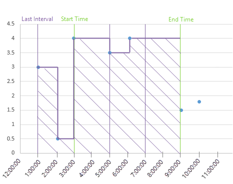
Ranged Average
This method returns a series of values determined via the Average method, spaced regularly between the Start Time and End Time according to the Interval parameter.
As with single point average, each value calculated from the time weighted average of raw data, and the returned timestamps are based on the request/interval time. The Interval parameter represents both the spacing of data, and the duration over which each average is calculated.
It is important to note that each time-weighted average represents the period before the timestamp; thus the first return value of a ranged average fetch actually represents data before the start time.
In the case of the example below, the integral (area) is calculated as follows:
- First interval (from the Start Time, back one Interval)
- Segment 1: area = 3 * 3600 seconds
- Segment 2: area = 0.5 * 3600 seconds
- Time weighted average = (10800 + 1800) / (3600 + 3600) = 1.75
- Second interval
- Segment 1: area = 4 * 7200 seconds
- Time Weighted Average = (28800) / (7200) = 4
- Third interval
- Segment 1: area = 3.5 * 3600 seconds
- Segment 2: area = 4 * 3600 seconds
- Time weighted average = (12600 + 14400) / (3600 + 3600) = 3.75
- Fourth interval (on the End Time)
- Segment 1: area = 4 (extrapolated from the datum at 6:00:00AM) * 7200 seconds
- Time Weighted Average = (28800) / (7200) = 4
Thus the parameters and return values are as follows:
Parameters: Start Time = 3:00:00 AM, End Time = 9:00:00 AM, Interval = 7200 seconds
Return values:
Response Value = 1.75, Timestamp = 3:00:00 AM
Response Value = 4, Timestamp = 5:00:00 AM
Response Value = 3.75, Timestamp = 7:00:00 AM
Response Value = 4, Timestamp = 9:00:00 AM
Single Point Fetch
With a Single Point Fetch, the start and end time are set to the same date/time (such as 2-1-2015) and only 1 point of data is returned. Single point fetches are most commonly used with the Last Known Value sample method.
In the background, a single point fetch will use the provided end date and automatically subtract the sample interval from it, to arrive at the start date. This saves the external application from having to calculate this itself. Other sample methods, such as average, will continue to function correctly. You can consider a single point fetch as being a smart helper when you only want a single value returned.
A single point fetch is typically used to display a single value on an Explorer page, for example on a schematic page. We only have the ability to display one number on the page, so there is no point in returning more data than we can show. In the following example, the source system has data for the specified time period. If there is no data for that period, no data points would be returned.
![]()
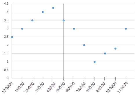
Single Point Raw
Single Point Raw sampling returns the last occurring value on or before the requested time, with the timestamp of the requested value.
If a value exists for the requested time, that value will be returned along with the timestamp of the value, as demonstrated in the following example.
Parameters: Request Time = 5:00:00 AM
Return values: Response Value = 3.5, Timestamp = 5:00:00 AM
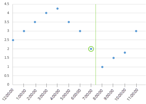
Single Point Raw - No Value
If no value exists for a requested time, then the last value before the requested time is returned, as demonstrated in the following example.
Parameters: Request Time = 7:30:00 AM
Return values: Response Value = 2, Timestamp = 7:00:00 AM
Single Point Last Known Value
Single Point Last Known Value sampling returns the last known value with the timestamp of the request (not the timestamp of the value).
This works much the same as Single Point Raw; however, in cases where no value exists for a requested time, the timestamp of the request itself is returned, instead of the timestamp of the requested source data.
If a value exists for the requested time, that value will be returned along with the timestamp of the request. For example:
Parameters: Request Time = 5:00:00 AM
Return values: Response Value = 3.5, Timestamp = 5:00:00 AM
Single Point Last Known Value - No Value
If no value exists for a requested time, then the last value before the requested time is returned, along with the timestamp of the request (as opposed to the timestamp of the source data). For example:
Parameters: Request Time = 7:30:00 AM
Return values: Response Value = 2, Timestamp = 7:30:00 AM
Single Point Linear Interpolate
Single Point Linear Interpolation calculates the intersection between the requested time and the interpolation of adjacent raw values.
If a value exists for the request time, no interpolation is required and that value will be returned along with the timestamp of the request. For example:
Parameters: Request Time = 5:00:00 AM
Return values: Response Value = 3.5, Timestamp = 5:00:00 AM
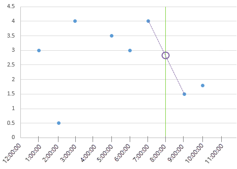
Single Point Linear Interpolate - No Value
If no value exists at the request time, a gradient between the first value occurring before and the first value occurring after the requested time is calculated, and the value found at the intersect of this line and the time requested is returned.
In the case of the example below, a line is drawn between the previous value of 4 at 6:00:00 AM, and the next value of 1.5 at 9:00:00 AM. The result is calculated by the intersection of the request time as follows:
Parameters: Request Time = 8:00:00 AM
Return values: Response Value = 2.333, Timestamp = 8:00:00 AM
Single Point Average
Single Point Average sampling calculates the time-weighted average for a particular point in time over the requested interval.
The idea behind time-weighting is that continuous-type data may have irregularly spaced data due to compression by historians. The absence of a raw datum does not mean that that value is less significant; instead it is assumed that the last value extrapolates forwards.
Mathematically, the time-weighted average is determined by calculating the integral of the data (the area under the curve), divided by the duration.
In the case of the example below, the integral (area) is calculated as follows:
Segment 1: area = 4 (extrapolated from the datum at 3:00:00AM) * 3600 seconds
Segment 2: area = 3.5 * 3600 seconds
Segment 3: area = 4 * 7200 seconds
Time Weighted Average = (14400 + 12600 + 28800) / (3600 + 3600 + 7200) = 3.875
Parameters: Request Time = 8:00:00 AM, Interval = 14400 seconds
Return values: Response Value = 3.875, Timestamp = 8:00:00 AM